II.2. Microstructure approach and uncertainty to
exchange rate determination
a. Concept of uncertainty
The concept of uncertainty may be divided in two forms where
we have the endogenous uncertainty and the exogenous uncertainty. The
endogenous uncertainty is based on the internal facts which can be seen
sometimes as technical uncertainty; we describe here the time factor of
uncertainty, the complexity of a project as a factor too, the intangible factor
of uncertainty such as switching on workforce productivity, rare labour in the
economy. On the endogenous uncertainty the paper describes also the financial
uncertainty such as cost and liquidity. And finally the paper has described the
product uncertainty such as the quality, the performance and the standard of
the market.
In the other hand the paper studies the exogenous uncertainty
as the external factors of uncertainty or market uncertainty which may be
partly internal depending on how much influence the ZAR/USD exchange rate has
in the foreign exchange market. Also it's describing the exogenous uncertainty
if there is a potential competitor of the ZAR or the USD and the quantity and
price of the supply and demand on the two countries. Finally another factor of
exogenous uncertainty is base on the specific region such as political risks,
war or conflict, regulation and environment.
b. Microstructure approach
Here the exchange rate tries to come out on a new approach
because most of the past macroeconomic approaches to exchange rate are
empirical failures. In 1995 (p1709) Frankel and Rose said: «to repeat a
central fact of life there is remarkably little evidence that macroeconomic
variable have consistent strong effects on floating exchange rate expect during
extraordinary circumstances such as hyperinflations.» Generally it's
agreed that fundamentals are explanatory over a long-term and fundamentals do
play a role in exchange rate determination but there is room of uncertainty in
mind.
In the asset market approach, the currency demand from
purchase and sale of assets as well, makes investor who wants to buy government
bonds or buy shares then must first buy currency and in addition to initial
demand for currency there is now also a view on future movement as the return
is paid in foreign currency; there is two alternatives; one for swap and the
other for order flow. That why we have the notion of information and
informational efficiency. On the evidence the asset approach models fail to do
better because it can't explain the volume in the foreign exchange market, it
doesn't have room for heterogeous beliefs and how does trading be translated
into price. The microeconomics is based on the order flow first where there is
quantity and the transaction volume, secondly on the spreads which provides the
price and finally it gives the stages of information processing.
III. METHODOLOGY
Most of the fundamental models were based on the linear
(parametric) time series modeling which offers a great wealth of modeling tools
in fact but also exhibit non stationary behaviour caused by the presence of the
unit roots, structural breaks, seasonal influences... And the fundamental
variables have been identified to explain the exchange rate over a long term;
which is more than five years data set both dependent and independent variables
with the same frequency. If there is a nonlinear dynamics, it's no longer
sufficient to consider linear models specifically the adjustment speed toward
long-run equilibrium of exchange rate is not proportional to the deviation. We
focus in the nonparametric estimation of univariate non linear model where it
may contain conditionally heteroskedastic errors and seasonal features;
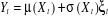
deferring seasonal models, we assume that a univariate stochastic process  is generated by the conditionally heteroskedastic nonlinear
autoregressive (NAR) model. is generated by the conditionally heteroskedastic nonlinear
autoregressive (NAR) model.
 (3.1) (3.1)
Where 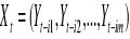 is the (mx1) vector of all m correct lagged values,
i1<i2<...<im, the ît S, t=im+1, im+2,..., denote a sequence of
iid random variables with zero mean and unit variance, and u
(.) and ó (.) denote the conditional
mean and volatility function, respectively. In this paper a nonlinear
autoregressive kernel model for a univariate time series is built in five
steps, namely, the estimation of the density function (Kernel function), the
search for an optimal bandwidth for kernel function, the determination of exact
number of lags to be included in the regression equation and the estimation of
the conditional mean and volatility. is the (mx1) vector of all m correct lagged values,
i1<i2<...<im, the ît S, t=im+1, im+2,..., denote a sequence of
iid random variables with zero mean and unit variance, and u
(.) and ó (.) denote the conditional
mean and volatility function, respectively. In this paper a nonlinear
autoregressive kernel model for a univariate time series is built in five
steps, namely, the estimation of the density function (Kernel function), the
search for an optimal bandwidth for kernel function, the determination of exact
number of lags to be included in the regression equation and the estimation of
the conditional mean and volatility.
The foreign exchange market modelling is typically associated
with large amounts of high dimensional data. The data typically has a low
signal to noise ratio and the signals are usually nonlinear. These problems
make financial market modeling particularly challenging. Wolberg (2000) argue
that kernel regression is particularly attractive for financial market
applications and can be used to develop models that do not rely on
distributional or functional assumptions. Use the exchange rate to assess the
forecasting power of the nonparametric kernel regression model.
Density estimation: in this paper the smooth
density function is known as the kernel estimator 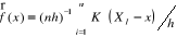 (3.2) (3.2)
Where: h is the smoothing parameter known as the bandwidth;
K(.) the kernel function chosen to be unimodal probability density which is
symmetric at zero. For instance, the kernel estimator has a value at a point x
which is the average of the n kernel ordinates at that point. In practice the
choice of the kernel function shape is less important than the choice of the
optimal bandwidth.
Optimal bandwidth selection: the integrated
mean squared error of the kernel estimator (imsef(x)) is used to obtain the
optimal bandwidth( John, MCom 2010).
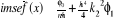 (3.3) (3.3)
Where:  and and  (3.4) (3.4)
The optimal bandwidth  can now be obtained by minimizing the imsef(x) above with respect to
the bandwidth h: can now be obtained by minimizing the imsef(x) above with respect to
the bandwidth h: 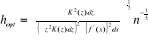 (3.5) (3.5)
Epanechnikov suggested the optimal kernel density estimator which corresponds with
the above optimal bandwidth: suggested the optimal kernel density estimator which corresponds with
the above optimal bandwidth: 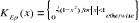 (3.6) (3.6)
Estimation of conditional mean and
volatility: Let  be the exchange rate at time t and be the exchange rate at time t and  the exchange rate in the previous periods. By assumption there is a
nonparametric relationship between the current and the previous exchange rate.
The nonlinear autoregressive heteroskedastic process is modelling as follow: the exchange rate in the previous periods. By assumption there is a
nonparametric relationship between the current and the previous exchange rate.
The nonlinear autoregressive heteroskedastic process is modelling as follow:
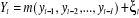 ; t=1,2,3,...T (3.7) ; t=1,2,3,...T (3.7)
Where:  and and 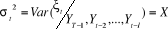 (3.8) (3.8)
The equation (3.7) represents the conditional mean and the
conditional volatility of the exchange rate is representing by . When we have to plot the conditional mean and volatility functions in
three-dimensional space, we assumed that only two lags have been selected for
prediction and the equation (3.7) may be rewritten as follows: . When we have to plot the conditional mean and volatility functions in
three-dimensional space, we assumed that only two lags have been selected for
prediction and the equation (3.7) may be rewritten as follows:
 (3.9) (3.9)
The equation (3.9) is different with the classical
autoregressive firstly in the sense it assumes a non-linear dependence on past
exchange rate and secondly it the classical GARCH models of volatility assume
normality and symmetrical behaviour while the distribution of exchange rate and
error terms doesn't have any such assumption.
The exchange rate data set and his optimal bandwidth selected
will have the estimator conditional mean denoted by ( where p is the degree of polynomial fitting of the exchange rate. The
Nadaraya-Watson conditional mean estimator is obtained when p is zero: where p is the degree of polynomial fitting of the exchange rate. The
Nadaraya-Watson conditional mean estimator is obtained when p is zero:  (3.10) (3.10)
IV. RESULTS
The study finds that the price exchange rate has little
forecasting power for rate changes when the forecast horizon is one year, but
its forecasting power increases significantly when the forecast horizon is more
than 3 years. The paper tries to compare two modes of forecasting where one is
the prediction based on Jmulti software and the other one based on the R
software.
The daily spot exchange rate have been used in Jmulti software
and selected from 03 January 2006 to 30 July 2010; The weekly exchange rate and
its spread have been used in R software and selected from the first week of
January 2001 to the last week of September 2010 in order to compare the
forecasting power of the kernel model, the root mean square error criterion as
well as the bootstrap confidence interval and the volatility are used.
a) Jmulti results
The paper divides the sample period in two consecutive
periods; the first is named in-sample, from 03 January 2006 to 11 May 2010 with
1091 observations, and the out-of-sample with 57 observations, from 11May 2010
to 30 July 2010.
The Epanechnikov Kernel has been used as the estimator of our
model density function corresponding to individual distribution of all the
ZAR/USD exchange rates (ask and bid prices). The paper used the automated
optimal bandwidth selection on JMulti software for lag selection as well as for
the estimation of conditional mean and volatility.
Two lags have been considered for the kernel regression and
the largest lags were five previous days. The local linear estimators of
conditional mean for the spot close exchange rates used lags one and three; the
previous day and the third previous day of exchange rate (lag one and three)
have been found to have a significant impact on the current rate. The
conditional volatility of the exchange rates is modelled using lag one and lag
five and both previous days of exchange rate have been found to have a
significant impact on the current volatility but the estimated volatility of
white noise process is very low.
To further the performance the F-Stat test is used and the
underlying idea is that, if the null hypothesis of an F-Stat is not rejected
then the method used to generate these forecasts is empirically good model to
generate future scenarios for long and short positions in the market.
The forecasts are generated using the kernel regression in two
methods; the first relies on one step ahead where the output of estimation
panel provides the prediction of the day after the 1091th
observation and the second is given on the rolling over method at 95% of
confidence of interval. The one step ahead prediction gives the conditional
values of 7.334 and 7.388 respectively for lag one and lag three. When plug-in
the bandwidth used for prediction in out-of-sample forecast the finding of an
interval of 7.19872 to 7.47507. the second gives the conditional value of 7.557
and 7.681 and Mean squared prediction error: 0.0046154052.
b) R Software
On the two variables in this application the paper visualise
the kernel density function of the ZAR/USD exchange rate and the spread of the
exchange rate. The distribution of our sample wasn't normal but when we
consider only the exchange rate from almost 6 Rands a USD to almost 9 Rands a
USD, we have a normal distribution. The rejection of the null hypothesis as
well as the non applicable of the predicted mean square error (pmse) discards
the dynamic of forecasting method in this study. The forecast below shows the
minimum and the maximum of the prediction and other important values.
Table 1: Forecast
|
Min.
|
1st Qu.
|
Median
|
Mean
|
3rd Qu.
|
Max.
|
|
7.37
|
7.096
|
7.329
|
7.623
|
7.848
|
10.6208.3.
|
Further investigation is needed to assess the performance of
kernel model when using R software over the Jmulti. In term of the confidence
interval for the thousand observations based on the predicted mean square error
criterion the kernel regression in Jmulti outperforms.
V. CONLUSION
In this paper we investigated the predictability of the
ZAR/USD exchange rate behaviour according to the current
exogenous and endogenous uncertainty by using a nonparametric (kernel) models.
The analysis was limited on the spot exchange rate (ask and bid prices). A
sample of one thousand and one hundred forty nine observations has been divided
in two periods namely the in-sample and the out-of-sample periods for the
Jmulti compare to R software with a sample of five hundred observations where
we associated the spread on the exchange rate. Firstly the paper analyses the
selection of the model and after that it proceeds on showing the volatility of
the foreign market in regard to the ZAR/USD was significantly influenced by the
previous trading and the trading from the first previous day and the third
previous day. Based on the predicted mean square error, the results suggest
that the prediction from one step ahead is closer to actual rates. The
prediction mean square error from the rolling over method is greater than that
from the one step ahead method.
References
1. Keith Cuthbertson, Quantitative financial economics; stocks,
bonds and foreign exchange, 1996, p 291-304
2. J. Frankel and Rose, Handbook of economics, 1995
3. Laurence S. Copeland Exchange rates and international finance,
, 1995, 2edition.
4. Epanechnikov, V., 1969. Nonparametric estimation for
multivariate probability densities. Theory Probab. Applic,14:153-158
5. J. Mwamba, Application of financial economics course, UJ,
MCom 2010
| 

