2.6 Conclusion
Throughout this chapter, we have studied an epidemiological
model. It follows from our study that infectious diseases can indeed be
characterized by mathematical models. These models allowed us to represent the
variation of the population in the form of differential equation systems, often
non-linear. It was a question for us to make the different stability analyses,
namely the analysis of the local stability of disease-free equilibrium (DFE),
and the global asymptotic stability of the disease-free equilibrium. One of the
most important criteria to characterize the diffusion of an epidemic is R
(Number of reproduction with control measures) which is the basic
reproduction rate of the virus during the epidemic taking into account the
control measures (social distancing, face mask, containment, case detection).
It appears that when R < 1 the DFE is globally asymptotically
stable and unstable when Rc > 1, the endemic
equilibrium when it exists is globally asymptotically stable for
Rc > 1 making automatically unstable the DFE
[24].
Master's thesis II * Molecular Atomic Physics and
Biophysics Laboratory-UYI * YAMENI STEINLEN DONAT D
(c)2021
CHAPTER III
RESULTS AND DISCUSSION
27
3.1 Introduction
The objective of this chapter is to present clearly the
results of the simulation of the system (2-2) by seeing the influence of
certain parameters of the model on the dynamics of the evolution of certain
compartments, to carry out a prediction for the case of Yaounde and Douala in
Cameroon and finally to evaluate the impact of the social distancing and the
use of the face mask.
3.2 Numerical method
In this section, we will perform sensitivity analysis on the
model parameters due to uncertainties involved in the estimation of some of the
model parameters. We will also perform numerical simulations of the model to
evaluate the impact of various control strategies on the disease dynamics. The
equations of the model (2-2) are solved numerically using the Matlab toolbox
ODE45 based on the Runge-Kutta fourth order method. The stability of the method
is well established in [28].
3.3 Model fitting
Cases are reported continuously from March 17, 2020,
Therefore, we consider March 17, 2020 as the start date of the epidemic in
Cameroon. We set the population size of Yaounde and Douala as the initial value
of the susceptible group (S(0) = 8 × 10⁶). The incubation
period of COVID-19 varies from 2 to 14 days, with an average of 5 to 7 days,
and we take the value of 7 days in our model. The average recovery period is
about 15 days[29], and so we set disease recovery rates at ó1 =
ó2 = 1/15 per day.
3.3. MODEL FITTING 28
Master's thesis II * Molecular Atomic Physics and
Biophysics Laboratory-UYI * YAMENI STEINLEN DONAT D
(c)2021
The model fitted to the accumulation of newly reported cases
is shown in Figure 3.1. The estimated parameter values are given in Table 2. It
can be seen from Figure 3.1 that the prediction of model (2.2) has a similar
trend to the reported cumulative conforming case data [4].
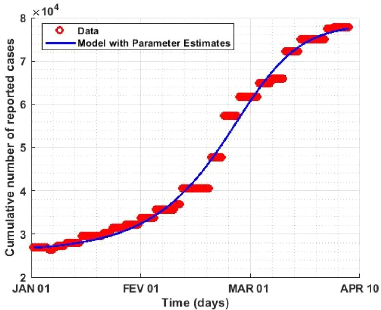
Figure 3.1: Model adapted to the new cumulative cases of COVID-19
reported for the period 01 January 2020 to 10 April 2021.
Figure (3.1) shows that our model fit well to the Cameroon data
(cumulative daily number of reported cases) for the period January 01, 2020 to
April 10, 2021. The blue curve represents the model solution and the red curve
represents the disease cases per day.
Table 2: Estimated parameters
3.4. MODEL SENSITIVITY ANALYSIS 29
Master's thesis II *
Molecular Atomic Physics and Biophysics Laboratory-UYI
* YAMENI STEINLEN DONAT D
(c)2021
|
Parameters
|
values
|
Sources
|
|
À
|
500
|
assumed
|
|
â1
|
0.7421
|
estimated
|
|
â2
|
0.0485
|
estimated
|
|
cf
|
0.0446
|
estimated
|
|
p
|
0.9150
|
estimated
|
|
ä
|
0.1428
|
assumed [29]
|
|
E
|
0.0096
|
estimated
|
|
u
|
0.0015
|
asusmed [30]
|
|
á
|
0.1473
|
estimated
|
|
u1
|
0.066
|
assumed [29]
|
|
u2
|
0.066
|
assumed [29]
|
|
è
|
0.2988
|
estimated
|
|
ø
|
0.19
|
estimated
|
3.4 Model sensitivity analysis
We do the sensitivity analysis around Rc, it is a
question of showing on the one hand the parameters which influence positively
the model, and those which influence negatively the model on the other hand.
Using the formula
n ?Rc
?n = .?n , (3.1)
Rc
Where n represents here the different parameters of our model,
we calculate the different indices of our model.
Table 2: Sensitivity indices of the model
3.4. MODEL SENSITIVITY ANALYSIS 30
|
Parameters
|
Index if sensitivity
|
|
À
|
1
|
|
â1
|
0.9748
|
|
â2
|
0.0252
|
|
cf
|
-1
|
|
p
|
0.7036
|
|
u
|
-0.2058
|
|
E
|
-0.0041
|
|
á
|
-0.5440
|
|
ó1
|
-0.2462
|
|
è
|
-0.4261
|
|
ø
|
-0.2372
|
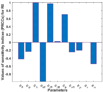
Figure 3.2: Histogram of the sensitivity analysis between
Rc and each parameter
Master's thesis II * Molecular Atomic Physics and
Biophysics Laboratory-UYI * YAMENI STEINLEN DONAT D
(c)2021
3.5. SHORT-TERM PREDICTIONS 31
Master's thesis II * Molecular Atomic Physics and
Biophysics Laboratory-UYI * YAMENI STEINLEN DONAT D
(c)2021
Because of the uncertainties that may arise in the parameter
estimates used in the simulations, a Latin hypercube sampling (LHS) [32] is
implemented on the model parameters. For the sensitivity analysis, we perform a
Partial Rank Correlation Coefficient (PRCC) between the values of the
parameters in the response function and the value of the response function
derived from the sensitivity analysis [33]. individual transmission rate /31,
the detected infection individual transmission rate /32, recovery
rate of infected individuals a1, recovery rate of quarantined individuals U2,
the accounting of parameters p, /31, /32, and a, have a positive
influence on Re, an increase of these parameters thus implies an
increase on Re. A when 0, B, a, E, a1, cf, and ,u have a negative
influence on Re; an increase in these parameters implies a decrease
in Re.
The public health implication is that, COVID-19 can be
effectively controlled in the population by reducing the rate of transmission,
achieved by preventive measures such as strict social distancing regulations
and mandatory wearing of masks in public, and also by reducing the
infectiousness of asymptomatic humans through appropriate treatment.
Furthermore, the disease burden can be significantly reduced in the population
if efforts are put in place to intensify the detection rates of asymptomatic
and symptomatic infectious humans in order to isolate them and offer them
appropriate treatment.
From this analysis, we can make the following suggestions:
* Mass screening is a good control tool because it increases
the value of the quarantine rate. * Boundary locking has proven to be an
effective control measure against the growth of COVID-19, as it reduces the
value of the susceptible recruitment rate.
* The containment rate of susceptible individuals contributes
to reducing the values of the transmission rates /31 and /32 and to
increasing cf, so this containment rate plays an important role in reducing the
number of infected individuals.
|