3.1.2.2 Planar array antenna
In addition to placing elements along a straight row to form a
linear array, individual
elements can be positioned along a rectangular grid to form a
rectangular or planar
array, which is capable of providing more variables for
controlling and modeling of
beam pattern. Moreover, planar arrays are also more versatile
with lower side lobe levels
and they can be used to scan the main beam of the antenna
towards any point in space.[6]
Referring to Fig 3.2, the array factor can be derived for a
planar array.
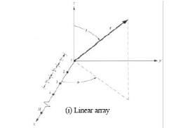
Fig
3.2: Linear and Planar geometries [6].
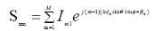
Placing M elements along the x-axis as shown
in Fig 3.2 (i) will have an array factor represented by
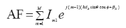 (3.3)
(3.3)
Where: Im1= Excitation coefficient of individual
element
dx= Inter element spacing along x-axis
âx = Progressive phase shift between
elements along x-axis
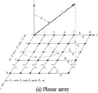
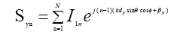
A rectangular array shown in Fig 3.2 (ii) will be formed if
N elements array with a
distance dy apart and with a progressive phase
ây, is placed in the y-direction. Thus, the
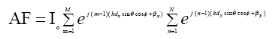
array factor for the entire planar array can be written
as[6]
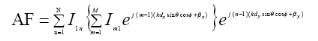 (3.4)
(3.4)
or,
 (3.5)
(3.5)
where
 (3.6)
(3.6)
 (3.7)
(3.7)
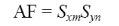
From equation (3.5), it can be seen that the pattern of a
rectangular array is the product of the array factors of the arrays in the
x- and y-plane.
The amplitude of the (m,n)th element can
be written as shown in equation (3.8) if the amplitude excitation coefficients
of the elements of the array in the y-direction are proportional to
those in the x [24],
 (3.8)
(3.8)
However, if the amplitude excitation of the array is uniform
(Imn = Io), then equation
(3.4) can be represented by
 (3.9)
(3.9)
and the normalized form will be
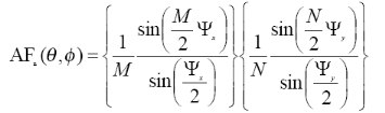 ( 3.10)
where,
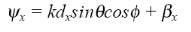 (3.11)
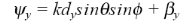 (3.12)
The above derivation assumed that each element is an isotropic
source. However, if the
antenna is an array of identical elements, the total field can
be obtained by applying the
pattern multiplication rule of (3.1) in a manner similar as
for the linear array [24].
| 

