implémentation d'une nouvelle méthode d'estimation de la matrice variance covariance basée sur le modèle GARCH multivarié, simulation par backtesting de stratégies d'investissement.

Conclusion générale

Au cours de la préparation de notre mémoire de fin d'études, nous avons été amenés à faire des prévisions à l'aide de diverses méthodes sur des séries financières. Et essayer d'attendre l'objectif principal de notre étude qui est de tester une nouvelle modélisation de la matrice de variance covariance pour l'optimisation de portefeuilles financiers.

Pour cela nous avons proposé dans un premier temps d'étudier individuellement les séries en utilisant l'approche univariée, cette approche nous a permis de représenter nos séries avec des modèles ARMA et ARIMA avec des résidus ARCH ou GARCH.

En suite on est passé à la méthode Holt & Winters, pour faire une prévision à court terme et comparer les résultats avec ceux de la méthodologie de Box et Jenkins.

En effet, l'application de ces deux méthodes sur des séries financières nous a permis de conclure que :

Les modèles ajustés ARMA (1,1) et ARMA (3,3) sont plus performant que celui de la méthode Holt & Winters pour les séries IEV et SPY qui représentent respectivement la valeur des actions de 350 sociétés les plus représentatives de l'économie européenne et la valeur des actions de 500 compagnies les plus représentatives de l'économie américaine.

Par contre, la méthode Holt & Winters semble meilleure que les modèles intégrés ARIMA (2, 1,0) et ARIMA (4, 1,4) des séries QQQQ et GLD qui représentent respectivement la valeur des actions des 100 plus grandes compagnies innovantes autre que financières et la valeur de l'OR sur les marchés internationaux.

Cependant la méthodologie de Box et Jenkins ne prend pas en compte l'interdépendance des séries, pour cette raison nous avons proposé par la suite une approche hétéroscédastique multivariée pour parer aux insuffisances de l'approche univariée.

Dans la partie multivariée, nous avons passé en revue les différentes méthodes utilisées dans l'estimation de la volatilité. Nous avons d'abord commencé par les différentes approches depuis leurs créations, la première approche est le modèle VEC proposé par Bollerslev, Engle et Wooldrige (1988), c'est une extension directe du modèle ARCH univarié, l'inconvénient majeur de ce modèle est le nombre de paramètres à estimer, il devient de plus en plus grand au fur et à mesure que le nombre des variables augmente. Pour réduire le nombre de paramètres à estimer, les auteurs suggèrent la formulation diagonale VEC (DVEC).

Certes, ce modèle réduit remarquablement le nombre de paramètres à estimer par rapport au modèle précédent, mais le grand désavantage de ce modèle est l'absence de l'interdépendance entre les composants du système donc la transmission de chocs entre les variables n'est pas possible. Les variations de la volatilité d'une variable n'influencent pas le comportement des autres variables dans le système. D'autre part, la positivité de la matrice des variances covariances conditionnelles n'est pas garantie par le modèle. Il faudrait imposer des restrictions sur chaque élément de la matrice des variances covariances conditionnelles.

Pour pallier aux insuffisances des modèles VEC et DVEC, une approche qui garantit la positivité de la matrice des variances covariances conditionnelles est suggérée par Baba, Engle, Kraft et Kroner (1 990).Puis elle a été synthétisée dans l'article d'Engle et Kroner (1995). Le modèle BEKK prend en compte des interactions entre les variables étudiées. Néanmoins, bien que le nombre des paramètres à estimer soit inférieur à celui des modèles VEC et DVEC, il demeure encore très élevé. Les recherches utilisant ce modèle limitent le nombre d'actifs étudiés et ou imposent des restrictions comme de supposer que les corrélations sont constantes.

On a commencé par une modélisation de la matrice variance covariance par la spécification CCC de Bollerslev (1990), en suite on a effectué un test de constance de corrélation pour passer au modèle DCC de Engle et Sheppard (2002). Le DCC GARCH de Engle et Sheppard (2002) a été retenu comme modèle économétrique de référence car il permet de réduire de manière significative le nombre de paramètres à estimer et il fournit une interprétation relativement simple des corrélations. Ce type de modèle GARCH est donc beaucoup plus rapide à implémenter et beaucoup plus convivial lorsque vient le moment d'interpréter les coefficients, c'est cela l'avantage qu'il offre aux professionnels de la finance.

Les résultats du modèle GARCH DCC ont été comparés en matière de gestion de portefeuille à ceux de la méthode de calcul empirique de la matrice de corrélation utilisée par la plupart des sociétés financières.

Cette comparaison a eu lieu grâce à une opération appelée dans le monde de la finance, le Backtesting. Cette opération, consiste à simuler dans le passé une stratégie d'allocation de portefeuille, c'est-à-dire une manière d'attribuer des poids à chacun des actifs du portefeuille au cours du temps. Elle permet en particulier, de vérifier de manière empirique, comment une stratégie donnée se serait comportée dans des conditions réelles en se plaçant dans le passé sur une période donnée.

Afin de comparer l'efficacité de l'optimisation en utilisant la méthode GARCH DCC, nous avons calculé la valeur du portefeuille en utilisant en parallèle une méthode d'optimisation quadratique (modèle mean-var de Markowitz) qui utilise une matrice de corrélation

empirique. Pour les deux méthodes, tous les paramètres d'optimisation étaient les mêmes mis a part la matrice de corrélation, on note aussi que lors des simulations par Backtesting on a fait l'hypothèse qu'il n'y a pas de coûts de transactions (ou qu'ils sont négligeables).

En fin on achève notre étude avec les résultats du Backtesting qui ont montré l'efficacité du modèle GARCH DCC par rapport à la méthode empirique, car ce modèle prend en compte la dynamique des volatilités des covariances et la fait introduire dans l'optimisation de portefeuille.

Le rendement du portefeuille GARCH DCC superforme nettement le rendement de la méthode empirique dans les périodes de forte volatilité, par contre dans les autres périodes il semble que les deux portefeuilles soient identiques, ce qui explique l'apport majeur de l'introduction de la dynamique entre les actifs dans l'optimisation de portefeuille.

Cette nouvelle méthode d'estimation de la matrice variance covariance est une nouvelle porte pour la gestion de portefeuilles financiers, car elle donne des résultats remarquables par rapports aux autres méthodes classiques et empiriques.

On espère avoir répondu aux problèmes posés et que les résultats trouvés seront d'une utilité pertinente surtout dans le monde de la gestion de portefeuilles financiers.

ANNEXE A : Symboles et Tableau

Symboles :

AR (p) Autorégressive processus of ordre p (processus autorégressive d'ordre p).

MA (q) moyenne mobile d'ordre q.

ARIMA (p, d, q) processus autorégressif moyenne mobile intégré d'ordre (p, d, q). GARCH(p, q) Generalised Autoregressif Conditional Heteroscedasticity

CCC Constant Conditional Correlation

DCC Dynamic Conditional Correlation

? Produit de Kronecker

AIC Akaike information.

SC Schwarz criterion.

E espérance.

e erreur.

Var variance.

MSE mean square error matrix (matrice de l'erreur quadratique moyenne).

T taille de l'échantillon ou longueur de la série chronologique.

BEKK Baba Engle Kraft et Kroner

Tables de Dikey Fuler

Valeurs critiques du test de Dickey Fuller pour p =1

T

1%

5%

10%

Modèle [1]

100	-2,6	-1,95	-1,61
250	-2,58	-1,95	-1,62
500	-2,58	-1,95	-1,62

Modèle [2]

100	-3,51	-2,89	-2,58
250	-3,46	-2,88	-2,57
500	-3,44	-2,87	-2,57

Modèle [3]

100	-4,04	-3,45	-3,15
250	-3,99	-3,43	-3,13
500	-3,98	-3,42	-3,13

Valeurs critiques de la constante et de la tendance :

Modèle [2]
Constante

	1%	5%	10%
100	3,22	2,54	2,17
250	3,19	2,53	2,16
500	3,18	2,52	2,16

RH ₀

AH ₀

p

A = #177; ? A #177; #177; #177;

X q X _ çb X ? J3 t C e

t t j t j

1 t

j ? 1

p

A = #177; ? A #177; #177;

X ? X ? ? X C e

t t j t j t

1 ?

j ? 1

A

p

X ? X ? çb X e

t t j t j t

= #177; A #177;

1 ?

j ? 1

AH ₀

R H0

AH ₀

AH ₀

R H0

RH₀

.

.

.

R H0

AH ₀

Modèle [3
Constante

	1%	5%	10%
100	3,78	3,11	2,73
250	3,74	3,09	2,73
500	3,72	3,08	2,72

Tendance

	1%	5%	10%
100	3,53	2,79	2,38
250	3,49	2,79	2,38
500	3,48	2,78	2,38

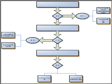
Algorithme de Dicky-Fuller augmenté :

Annexe B: Programmes Matlab

GARCH univarié:

function [parameters, likelihood, ht, stderrors, robustSE, scores, grad] = garchpq(data , p , q , startingvals, options)

% PURPOSE:

% GARCH(P,Q) parameter estimation with normal innovations using

analytic derivatives

%

% USAGE:

% [parameters, likelihood, ht, stderrors, robustSE, scores, grad] =

garchpq(data , p , q , startingvals, options)

%

% INPUTS:

% data: A single column of zero mean random data, normal or not for

quasi likelihood

%

% P: Non-negative, scalar integer representing a model order of the
ARCH

% process

%

% Q: Positive, scalar integer representing a model order of the GARCH

% process: Q is the number of lags of the lagged conditional

variances included

% Can be empty([] ) for ARCH process

%

% startingvals: A (1+p+q) vector of starting vals. If you do not
provide, a naieve guess of 1/(2*max(p,q)+1) is

% used for the arch and garch parameters, and omega is set to make

the real unconditional variance equal

% to the garch expectation of the expectation.

%

% options: default options are below. You can provide an options
vector. See HELP OPTIMSET

%

% OUTPUTS:

% parameters : a [ 1+p+q X 1] column of parameters with omega, alpha1,

alpha2, ..., alpha(p)

% beta1, beta2, ... beta(q)

%

% likelihood = the loglikelihood evaluated at he parameters

%

% ht = the estimated time varying VARIANCES

%

% stderrors = the inverse analytical hessian, not for quasi maximum
liklihood

%

% robustSE = robust standard errors of form A^-1*B*A^-1*T^-1

% where A is the analytic hessian

% and B is the covariance of the scores

%

% scores = the list of T scores for use in M testing

%

% grad = the average score at the parameters

%

% COMMENTS:

%

% GARCH(P,Q) the following(wrong) constratins are used(they are right for
the (1,1) case or any Arch case

% (1) Omega > 0

% (2) Alpha(i) >= 0 for i = 1,2,...P

% (3) Beta(i) >= 0 for i = 1,2,...Q

% (4) sum(Alpha(i) + Beta(j)) < 1 for i = 1,2,...P and j = 1,2,...Q

%

% The time-conditional variance, H(t), of a GARCH(P,Q) process is modeled

% as follows:

%

% H(t) = Omega + Alpha(1)*r_{t-1}^2 + Alpha(2)*r_{t-2}^2 +...+

Alpha (P)*r_{ t-p} ^2+...

% Beta(1)*H(t-1)+ Beta(2)*H(t-2)+...+ Beta(Q)*H(t-q)

%

% Default Options

%

% options = optimset('fmincon');

% options = optimset(options , 'TolFun' , 1e-003);

% options = optimset(options , 'Display' , 'iter');

% options = optimset(options , 'Diagnostics' , 'on');

% options = optimset(options , 'LargeScale' , 'off');

% options = optimset(options , 'MaxFunEvals' ,

'400* numberOfVariables');

% options = optimset(options , 'GradObj' , 'on');

%

%

% uses GARCH_LIKELIHOOD and GARCHCORE. You should MEX, mex 'path\garchcore.c', the MEX source

% The included MEX is for R12, 12.1 and 11 Windows and was compiled with Intel Compiler 5.01.

% It gives a 10-15 times speed increase

%

% Author: Kevin Sheppard

% [e-mail]

% Revision: 2 Date: 12/31/2001

if size(data,2) > 1

error('Data series must be a column vector.') elseif isempty(data)

error('Data Series is Empty.')

end

if (length(q) > 1) | any(q < 0)

error('Q must ba a single positive scalar or an empty vector for ARCH.') end

if (length(p) > 1) | any(p < 0)

error('P must be a single positive number.') elseif isempty(p)

error('P is empty.')

end

if isempty(q)

q=0; m=p; else m = max(p,q);

end

if nargin<=3 | isempty(startingvals)

guess = 1/(2*m+1);

alpha = .15*ones(p,1)/p;
beta = .75*ones(q,1)/q;

omega = (1-(sum(alpha)+sum(beta)))*cov(data); %set the uncond = to its e xpe c t ion

else

omega=startingvals (1);

alpha=startingvals (2:p+1);

beta=startingvals (p+2:p+q+1);

end

LB = [];

UB = [];

sumA = [-eye(1+p+q); ... 0 ones(1,p) ones(1,q)];

sumB = [zeros(1+p+q,1);... 1];

if (nargin <= 4) | isempty(options) options = optimset('fmincon');

options = optimset(options , 'TolFun' , 1e-003);

options = optimset(options , 'Display' , 'iter');

options = optimset(options , 'Diagnostics' , 'on'); options = optimset(options , 'LargeScale' , 'off'); options = optimset(options , 'MaxFunEvals' , 400* (1+p+q)); options = optimset(options , 'GradObj' , 'on');

end

sumB = sumB - [ zeros(1+p+q,1); 1]*2*optimget(options, 'TolCon', 1e-6);

stdEstimate = std(data,1);

data = [ stdEstimate(ones(m,1)) ; data];

% Estimate the parameters.

[parameters, LLF, EXITFLAG, OUTPUT, LAMBDA, GRAD] = fmincon('garchlikelihood', [omega ; alpha ; beta] ,sumA , sumB ,[] , [] , LB , UB,[] ,options,data, p , q, m, stdEstimate);

if EXITFLAG<=0

EXITFLAG

fprintf(1,'Not Sucessful! \n') end

parameters(find(parameters < 0)) = 0;

parameters(find(parameters(1) <= 0)) = realmin;

if nargout>1

[likelihood, grad, hessian, ht, scores, robustSE] = garchlikelihood(parameters , data , p , q, m, stdEstimate); stderrors=hessian^ (-1);

likelihood=-likelihood; end.

%%%%%%%%%%%%%%%%%%%%%% Fin du programme%%%%%%%%%%%%%%%%%%%%%%%%%%%%%%%%%

GARCH multivarié CCC (CCC-MVGARCH) :

function [parameters, loglikelihood, R ,Ht, likelihoods, stdresid, unistdresid, hmat, stderrors, A, B,

j ointscores] =cc _mvgarch (data, archP, garchQ)

% PURPOSE:

% Estimates a multivariate GARCH model using Bollerslev's constant

correlation estimator

%

% USAGE:

% [parameters, loglikelihood, R, Ht, likelihoods, stdresid,

unistdresid, hmat, stderrors, A, B, jointscores] =...

% cc_mvgarch (data, archP, garchQ)

%

% INPUTS:

% data: A zero mean t by k vector of residuals from some filtration

% archP: One of three things: Empty in which case a 1 innovation
model is estimated for each series

% A scalar, p in which case a p

innovation model is estimated for each series

% A k by 1 vector in which case the

ith series has innovation terms p=archP(i)

% garchQ: One of three things: Empty in which case a 1 GARCH lag

is used in estimation for each series

% A scalar, q in which case a q

GARCH lags is used in estimation for each series

% A k by 1 vector in which case the

ith series has lagged variance terms q=archQ(i)

%

% OUTPUTS:

% parameters= A vector of parameters estimated form the model of the

fo rm

% [GarchParams (1) GarchParams (2) ... GarchParams (k)

Correlation(ccvech of the correlation matrix)]

% where the garch parameters from each estimation are of

the form

% [omega(i) alpha(i1) alpha(i2) ... alpha(ip(i)) beta(i1)

beta(i2) ... beta(iq(i))]

% loglikelihood=The log likelihood evaluated at the optimum

% R = k x k matrix of correlations

% Ht= A k by k by t array of conditional variances

% likelihoods = the estimated likelihoods t by 1

% stdresid = The multivariate standardized residuals

% unistdresid = Residuals standardized by their estimated std devs

% Hmat = The t by k matrix of conditional variances

% stderrors=A length(parameters)^2 matrix of estimated correct

standard errors

% A = The estimated A form the rebust standard errors

% B =the estimated B from the standard errors

% scores = The estimated scores of the likelihood t by

length (parameters)

%

% COMMENTS:

% % % Author: Kevin Sheppard

% [e-mail]

% Revision: 2 Date: 12/31/2001

% Lets do some error checking and clean up [t, k] =size (data);

if k<2

error('Must have at least 2 data series') end

if ~(isempty(archP) | length(archP)==1 | length(archP)==k) error('Wrong size for archP')

end

if ~(isempty(garchQ) | length(garchQ)==1 | length(garchQ)==k) error('Wrong size for garchQ')

if isempty(archP)

archP=ones (1,k);

elseif length(archP)==1 archP=ones (1,k)*archP; end

if isempty(garchQ)

garchQ=ones (1,k);

elseif length (garchQ) ==1 garchQ=ones (1, k)*garchQ; end

% Now lest do the univariate garching using fattailed_garch as it's faster then garchpq

stdresid=data;

options=optimset ( 'fmincon');

options=optimset (options, 'Display','off', 'Diagnostics','off', 'MaxFunEvals', 1000*max(archP+garchQ+1), 'MaxIter' ,1000*max(archP+garchQ+1), 'LargeScale', 'o ff', 'MaxSQPIter' ,1000);

options = optimset(options , 'MaxSQPIter' , 1000);

hmat=zeros (t, k);

for i=1:k

fprintf(1,'Estimating GARCH model for Series %d\n',i)

[univariate{ i} .parameters, univariate{ i} .likelihood,

univariate{i} .stderrors, univariate{i} .robustSE, univariate{i} .ht, univariate{ i} .scores] ...

= fattailed_garch(data(:,i) , archP(i) , garchQ(i) , 'NORMAL',[], options); stdresid(:,i)=data(:,i)./sqrt(univariate{i} .ht);

hmat(:,i)=univariate{ i} .ht;

end

unistdresid=stdresid;

% The estimated parameters are real easy

R=corrcoef (stdresid);

% We now have all of the estimated parameters parameters=[ ];

H=zeros (t, k);

for i=1:k

parameters=[ parameters;univariate{ i} .parameters]; H(:,i)=univariate{ i} .ht;

end

parameters=[ parameters;ccvech(R)];

%We now have Ht and the likelihood

if nargout >=2

[loglikelihood, likelihoods] =cc _mvgarch _full _likelihood (parameters, data, archP,garchQ);

likelihoods=-likelihoods;

loglikelihood=-loglikelihood;

Ht=zeros (k, k, t); stdresid=zeros (t, k);

Hstd=H.^ (0.5); for i=1:t

Ht(:, :,i)=diag(Hstd(i, :))*R*diag(Hstd(i, :)); stdresid(i,:)=data(i,:)*Ht(:,:,i)^(-0.5);

end

if nargout>=9

%How ar we going to get STD errors? Partitioned invers probably. Well, we need to get the scores form the dcc model, the joint likelihood.

%We then need to get A12 and A22 so we can have it all. We also need to get A11 in the correct form.

A=zeros (length(parameters) ,length(parameters));

index=1;

for i=1:k

workingsize=size (univariate{ i} . stderrors);

A (index: index+workingsize-1, index: index+workingsize-

1)=univariate{ i} .stderrors^ (-1);

index=index+workingsize;

end

% Ok so much for a All and A12 and A22, as we have them all between whats above

fprintf(1,'\n\nCalculating Standard Errors, this can take a while\n'); otherA=dcc_hessian('cc_mvgarch_full_likelihood' ,parameters, (k* (k-1) /2), data, archP,garchQ);

A(length(parameters)-(k* (k-1)/2)+1:length(parameters), :)=otherA;

% tempA=hessian _2sided('dcc _garch _full _likelihood' ,parameters, data,

archP, garchQ, dccP, dccQ);

% A(length(parameters)-1 :length(parameters), : )=tempA(length(parameters)-

1 : length (parameters),:); %That finishes A

% We now need to get the scores for the DCC estimator so we can finish B jointscores=zeros (t,length(parameters));

index=1;

for i=1:k

workingsize=size (univariate{ i} . scores, 2);

jointscores (:, index:index+workingsize-1)=univariate{ i} . scores; index=index+workingsize;

end

%Now all we need to do is calculate the scores form teh dcc estimator and we have everything

h=max(abs(parameters/2) ,1e-2)*eps^(1/3);

hplus=parameters+h;

hminus=parameters-h;

likelihoodsplus=zeros (t,length(parameters));

likelihoodsminus=zeros (t,length(parameters));

for i=length(parameters)-(k* (k-1)/2)+1:length(parameters) hparameters=parameters;

hparameters (i) =hplus (i);

[HOLDER, indivlike] = cc_mvgarch_full_likelihood(hparameters, data, archP,garchQ);

likelihoodsplus (:, i)=indivlike;

end

for i=length(parameters)-(k* (k-1)/2)+1:length(parameters) hparameters=parameters;

hparameters (i) =hminus (i);

[HOLDER, indivlike] = cc_mvgarch_full_likelihood(hparameters, data, archP,garchQ);

likelihoodsminus (:, i)=indivlike;

end

CCscores=(likelihoodsplus(:,length(parameters)-(k* (k1)/2)+1:length(parameters))-likelihoodsminus(: ,length(parameters)-(k* (k-

1) /2) +1: length (parameters)))... ./(2*repmat(h(length(parameters)-(k* (k-1)/2)+1:length(parameters)) ',t,1)); jointscores(: ,length(parameters)-(k* (k-

1) /2) +1: length (parameters) ) =CCscores;

B=cov (jointscores);

stderrors=A^ (-1)*B*A^ (-1)*t;

end %Done!

%%%%%%%%%%%%%%%%%%%%%%%%%%%%%%%%%%%%%%%%%%%%%%%%%%%%%%%%%%%%%%%%%%%%%%%%%%%

%%%%%%%%%%%%%%%%%%%%%%%%%%%%%%%%%%%%%%%%%%%%%%%%

% Helper Function

%%%%%%%%%%%%%%%%%%%%%%%%%%%%%%%%%%%%%%%%%%%%%%%%%%%%%%%%%%%%%%%%%%%%%%%%%%%

%%%%%%%%%%%%%%%%%%%%%%%%%%%%%%%%%%%%%%%%%%%%%%%%

function [parameters] =ccvech (CorrMat)

[k, t] =size (CorrMat);

parameters=zeros (k* (k-1) /2,1);

index=1;

for i=1:k

for j=i+1:k

parameters (index) =CorrMat (i, j);

index=index+1;

end end

%%%%%%%%%%%%%%%%%%%%%%%%%%%%%%%%%%%%%%%%%%%%%%%%%%%%%%%%%%%%%%%%%%%%%%%%%%%

%%%%%%%%%%%%%%%%%%%%%%%%%%%%%%%%%%%%%%%%%%%%%%%%

%%%%%%%%%%%%%%%%%%%%%%%%%%%%%%%%%%%%%%%%%%%%%%%%%%%%%%%%%%%%%%%%%%%%%%%%%%%

%%%%%%%%%%%%%%%%%%%%%%%%%%%%%%%%%%%%%%%%%%%%%%%%

% Helper Function

%%%%%%%%%%%%%%%%%%%%%%%%%%%%%%%%%%%%%%%%%%%%%%%%%%%%%%%%%%%%%%%%%%%%%%%%%%%

%%%%%%%%%%%%%%%%%%%%%%%%%%%%%%%%%%%%%%%%%%%%%%%%

function [CorrMat] =ccivech(params)

[k, t] =size (params);

for i=2:m

if (k/((i* (i-1))/2))==1

sizes=i;

break

end

end

index=1;

CorrMat=eye (sizes)

for i=1:sizes

for j=i+1:sizes

CorrMat (i, j ) =params (index); CorrMat (j,i) =params (index); index=index+1;

end

end

%%%%%%%%%%%%%%%%%%%%%% Fin du programme% % % % % % % % % % % % % % % % % % % % % % % % % % % % % % % % %

Test de Engle et Sheppard:

function [pval, stat] =dcc_mvgarch_test(data,archP,garchQ,nlags); % PURPOSE:

% Test for presence of dynamic correlation

%

% USAGE:

% [pval, stat] =dcc_mvgarch_test(data,archP,garchQ,nlags);

% INPUTS:

% data - T by k matrix of residuals to be tested or dynamic

corrrelation

% archP - The length of the news terms in each univariate garch(either

a scalar or a k by 1 vector)

% garchQ - The length of the smoothing terms in each univariate

garch(either a scalar or a k by 1 vector)

% nlags - THe number of lags to use in the test

%

% OUTPUTS:

% pval - The probability the correlation is constant

% stat - The Chi^2 stat, with nlags+1 D.F>

%

% COMMENTS:

% % % Author: Kevin Sheppard

% [e-mail]

% Revision: 2 Date: 12/31/2001

[t, k] =size (data);

if isempty(archP)

archP=ones (1,k);

elseif length(archP)==1 archP=ones (1,k)*archP; end

if isempty(garchQ)

garchQ=ones (1,k);

elseif length (garchQ) ==1 garchQ=ones (1, k)*garchQ; end

[holder,holder2,holder3,holder4,holder5, stdresid] =cc _mvgarch(data,archP, gar chQ);

outerprods=[];

for i=1:k

for j=i+1:k;

outerprods=[ outerprods stdresid(:,i) .*stdresid(:,j)];

end
end

j=size (outerprods, 2);

regressors=[];

regressand=[];

for i=1:j

[Y,X] =newlagmatrix(outerprods (:, i) ,nlags, 1);

regressors=[ regressors; X]; regressand=[ regressand; Y]; end

beta=regressors\ regressand; XpX=(regressors'*regressors); e=regressand-regressors* beta; sig=e'*e/ (length(regressors-nlags-1));

stat=beta'*XpX*beta/sqrt (sig); pval=1-chi2cdf(stat,nlags+1); end.

%%%%%%%%%%%%%%%%%%%%%% Fin du programme% % % % % % % % % % % % % % % % % % % % % % % % % % % % % % % % %

GARCH multivarié DCC (DCC-MVGARCH) :

function [parameters, loglikelihood, Ht, Qt, stdresid, likelihoods, stderrors, A,B, jointscores] =dcc_mvgarch(data,dccP,dccQ,archP,garchQ)

% PURPOSE:

% Estimates a multivariate GARCH model using the DCC estimator of

Engle and Sheppard

%

% USAGE:

% [parameters, loglikelihood, Ht, Qt, likelihoods, stdresid,

stderrors, A,B, jointscores]...

% =dcc_mvgarch (data, dccP, dccQ, archP, garchQ)

%

% INPUTS:

% data = A zero mean t by k vector of residuals from some

filtration

% dccP = The lag length of the innovation term in the DCC

estimator

% dccQ = The lag length of the lagged correlation matrices in

the DCC estimator

% archP = One of three things: Empty in which case a 1

innovation model is estimated for each series

% A scalar, p in which case a p

innovation model is estimated for each series

% A k by 1 vector in which case the

ith series has innovation terms p=archP(i)

% garchQ = One of three things: Empty in which case a 1

GARCH lag is used in estimation for each series

% A scalar, q in which case a q

GARCH lags is used in estimation for each series

% A k by 1 vector in which case the

ith series has lagged variance terms q=archQ(i)

%

% OUTPUTS:

% parameters = A vector of parameters estimated form the model of

the form

% [GarchParams (1) GarchParams (2) ...

GarchParams (k) DCCParams]

% where the garch parameters from each estimation

are of the form

% [omega(i) alpha(i1) alpha(i2) ... alpha(ip(i))

beta(i1) beta(i2) ... beta(iq(i))]

% loglikelihood = The log likelihood evaluated at the optimum

% Ht = A k by k by t array of conditional variances

% Qt = A k by k by t array of Qt elements

% likelihoods = the estimated likelihoods t by 1

% stderrors = A length(parameters)^2 matrix of estimated correct

standard errors

% A = The estimated A form the rebust standard errors

% B = The estimated B from the standard errors

% scores = The estimated scores of the likelihood t by

length (parameters)

% % % COMMENTS:

% % % Author: Kevin Sheppard

% [e-mail]

% Revision: 2 Date: 12/31/2001

% Lets do some error checking and clean up [t, k] =size (data);

if k<2

error('Must have at least 2 data series')

end

if length (dccP) ~=length (dccQ) | length (dccP)~=1 error('dccP and dccQ must be scalars')

end

if ~(isempty(archP) | length(archP)==1 | length(archP)==k) error('Wrong size for archP')

end

if ~(isempty(garchQ) | length(garchQ)==1 | length(garchQ)==k) error('Wrong size for garchQ')

end

if isempty(archP)

archP=ones (1,k);

elseif length(archP)==1 archP=ones (1,k)*archP; end

if isempty(garchQ)

garchQ=ones (1,k);

elseif length (garchQ) ==1 garchQ=ones (1, k)*garchQ; end

% Now lest do the univariate garching using fattailed_garch as it's faster then garchpq

stdresid=data;

options=optimset ( 'fmincon');

options=optimset (options, 'Display','off', 'Diagnostics','off', 'MaxFunEvals', 1000*max(archP+garchQ+1), 'MaxIter' ,1000*max(archP+garchQ+1), 'LargeScale', 'o ff', 'MaxSQPIter' ,1000);

options = optimset(options , 'MaxSQPIter' , 1000);

for i=1:k

% fprintf(1,'Estimating GARCH model for Series %d\n',i)

[univariate{ i} .parameters, univariate{ i} .likelihood,

univariate{i} .stderrors, univariate{i} .robustSE, univariate{i} .ht, univariate{ i} .scores] ...

= fattailed_garch(data(:,i) , archP(i) , garchQ(i) , 'NORMAL',[], options); stdresid(:,i)=data(:,i)./sqrt(univariate{i} .ht);

end

options=optimset ( 'fmincon');

%options = optimset(options , 'Display' , 'iter');

%options = optimset(options , 'Diagnostics' , 'on'); options = optimset(options , 'LevenbergMarquardt' , 'on'); options = optimset(options , 'LargeScale' , 'off');

dccstarting=[ ones(1,dccP)* .01/dccP ones(1,dccQ)* .97/dccQ]; %fprintf(1, '\n\nEstimating the DCC model\n')

[dccparameters,dccllf,EXITFLAG,OUTPUT,LAMBDA,GRAD] =fmincon('dcc_mvgarch_lik elihood' ,dccstarting,ones (size(dccstarting)),[ 1-

2*options.TolCon] ,[] ,[] ,zeros(size(dccstarting))+2*options.TolCon,[] ,[] ,opt ions, stdresid,dccP,dccQ);

% We now have all of the estimated parameters

parameters=[ ];

H=zeros (t, k);

for i=1:k

parameters=[ parameters;univariate{ i} .parameters]; H(:,i)=univariate{ i} .ht;

end

parameters=[ parameters;dccparameters'];

%We now have Ht and the likelihood

[loglikelihood, Rt, likelihoods,

Qt] =dcc_mvgarch_full_likelihood(parameters, data, archP,garchQ,dccP,dccQ); likelihoods=-likelihoods;

loglikelihood=-loglikelihood;

Ht=zeros (k, k, t);

stdresid=zeros (t, k);

Hstd=H.^ (0.5);

for i=1:t

Ht(:,:,i)=diag(Hstd(i,:))*Rt(:,:,i)*diag(Hstd(i,:)); stdresid(i,:)=data(i,:)*Ht(:,:,i)^(-0.5);

end

save tempHt Ht

clear Ht

if nargout >=7

%How ar we going to get STD errors? Partitioned invers probably. Well, we need to get the scores form the dcc model, the joint likelihood.

%We then need to get A12 and A22 so we can have it all. We also need to get A11 in the correct form.

A=zeros (length(parameters) ,length(parameters));

index=1;

for i=1:k

workingsize=size (univariate{ i} . stderrors);

A (index: index+workingsize-1, index: index+workingsize-

1)=univariate{ i} .stderrors^ (-1);

index=index+workingsize;

end

% Ok so much for a All and A12 and A22, as we have them all between whats above

% fprintf(1,'\n\nCalculating Standard Errors, this can take a while\n');

otherA=dcc_hessian ( 'dcc _mvgarch _full _likelihood' ,parameters, dccP+dccQ, data, archP,garchQ,dccP,dccQ);

A(length(parameters)-dccP-dccQ+1 :length(parameters), : )=otherA;

% tempA=hessian('dcc _garch _full _likelihood' ,parameters, data,

archP, garchQ, dccP, dccQ);

% A(length(parameters)-1 :length(parameters), : )=tempA(length(parameters)-

1 : length (parameters),:); %That finishes A

% We now need to get the scores for the DCC estimator so we can finish B jointscores=zeros (t,length(parameters));

index=1;

for i=1:k

workingsize=size (univariate{ i} . scores, 2);

jointscores (:, index:index+workingsize-1)=univariate{ i} . scores; index=index+workingsize;

end

%Now all we need to do is calculate the scores form teh dcc estimator and we have everything

h=max(abs(parameters/2) ,1e-2)*eps^(1/3);

hplus=parameters+h;

hminus=parameters-h;

likelihoodsplus=zeros (t,length(parameters));

likelihoodsminus=zeros (t,length(parameters));

for i=length (parameters) -dccP-dccQ+1 : length (parameters) hparameters=parameters;

hparameters (i) =hplus (i);

[HOLDER, HOLDER1, indivlike] = dcc _mvgarch _full _likelihood(hparameters, data, archP,garchQ,dccP,dccQ);

likelihoodsplus (:, i)=indivlike; end

for i=length (parameters) -dccP-dccQ+1 : length (parameters) hparameters=parameters;

hparameters (i) =hminus (i);

[HOLDER, HOLDER1, indivlike] = dcc _mvgarch _full _likelihood(hparameters, data, archP,garchQ,dccP,dccQ);

likelihoodsminus (:, i)=indivlike; end

DCCscores= (likelihoodsplus (:, length (parameters) -dccP-

dccQ+1 : length (parameters) ) -likelihoodsminus (:, length (parameters) -dccPdccQ+1:length(parameters)))...

./(2*repmat(h(length(parameters)-dccP-dccQ+1:length(parameters)) ',t,1));

j ointscores (:, length (parameters) -dccP-dccQ+1 : length (parameters) ) =DCCscores; B=cov (jointscores);

A=A/t;

stderrors=A^ (-1)*B*A'^ (-1)*t^ (-1); end

%Done!

load tempHt

end.

%%%%%%%%%%%%%%%%%%%%%% Fin du programme% % % % % % % % % % % % % % % % % % % % % % % % % % % % % % % % %

Bibliographie

A. Ouvrages

1. BOSQ Denis, Jean- pierre LECOUTURE « Analyse et Prévision des séries chronologiques Méthodes paramétriques et non paramétriques »

2. Bourbonnais .régis : « Econométrie », ^4ème édition Dunod, Paris 2002.

3. Bourbonnais régis - Michel Terraza : « Analyse des séries temporelles », édition Dunod, Paris 2004.

4. Bourbonnais régis - Usunier Jean Claude : « Prévision des ventes », ^3ème édition Economica, Paris 2001.

5. Bollerslev, T. et E. Ghysels (1996), « Periodic AutoRegressive Conditional Heteroscedasticity »,Journal of Business and Economics, 14(2) :139-52.

6. Bollerslev, T., R.Y. Chou et K. F. Kroner (1992), « ARCH modeling in finance: A review of the theory and empirical evidence », Journal of Economics, 52:5-59.

7. Boullerslev, T. (1990), «Generalized AutoRegressive Conditional Heterosedasticity »

8. Charpentier Arthur: « Cours de séries temporelles théorie et applications », édition université Paris DAUPHINE. Larousse illustré, édition librairie Larousse 1984.

9. Capéraà Philippe - Bernard van Cutsen « Méthodes et modèles en statistique non paramétrique », édition Dunod, Paris 1988.

10. Cappiello, Engle and Sheppard, 2002, Asymmetric Dynamics in the Correlations of International Equity and Bond Returns», UCSD Discussion Paper, Correlations between 34 International equity and bond indices.

11. Dominick, (1986), «Econométrie et statistique appliquée », Serie Schaum.

12. DROSBERKE Jean jacques, BERNARD FICHET, PHILIPPE TASSI

« M ODEL ISATION ARCH », théorie statistique et applications dans le domaine de la finance.

13. Engle, 2002 : »Dynamic Conditional Correlation-A Simple Class of Multivariate GARCH Models», Journal of Business and Economic Statistics, Bivariate examples and Monte Carlo.

14. Engle and Sheppard, 2002 «Theoretical and Empirical Properties of Dynamic Conditional Correlation Multivariate GARCH», NBER Discussion Paper, and UCSD DP, Models of 30 Dow Stocks and 100 S&P Sectors.

15. Engle, R. F. et K. F. Kroner (1995), « Multivariate simultaneous generalized ARCH », Economet. Theory, 11 :122-50.

16. Engle R obert F. "A Note on Robust Methods for ARIMA Models, " in Applied Time Series Analysis of Economic Data, ed. A. Zellner (Washington, D. C.: Bureau of the Census, 1981), pp. 176-1 77.

17. Engle Robert F. "Multiperiod forecast error variances of inflation estimated from ARCH models, " (with Dennis Kraft), in Applied Time Series Analysis of Economic Data, ed. A. Zellner (Washington, D.C.: Bureau of the Census, 1983), 293-302.

18. Engle Robert F. "ARCH Models in Finance," (eds. R. Engle and M. Rothschild), Journal of Econometrics 52 (1992): 245-266.

19. Engle Robert F. "Editors Introduction" (with M. Rothschild), ARCH Models in Finance, eds. R. Engle and M. Rothschild, Journal of Econometrics 52 (1992): 1.

20. Engle Robert F. «Time Varying Volatility and the Dynamic Behavior of the Term Structure," (with V. Ng), Journal of Money, Credit and Baning 25 (1993): 336-349.

21. Engle Robert F. "Statistical Models for Financial Volatility, é» Financial Analysts Journal (Jan/Feb 1993): 72 - 78.

22. Engle Robert F. "ARCH Models, " (with D. Nelson and T. Bollerslev) in Handbook of Econometrics, Volume IV, ed. R. Engle and D. McFadden (Amsterdam: North Holland, 1994), 2959-3038. (without Figures 3 and 4).

23. Engle Robert F. «Forecasting Volatility and Option Prices of the S&P 500 Index," (with Jaesun Noh and Alex Kane), Journal of Derivatives 2(1994): 17-30.

24. Engle Robert F. «Multivariate Simultaneous GARCH," (with K. Kroner), Econometric Theory 11 (1995): 122-150.

25. Engle Robert F. "Estimating Common Sectoral Cycles," (with J. Issler), Journal of Monetary Economics 35 (1995): 83-113.

26. Engle Robert F. "GARCH Gammas," (with Joshua Rosenberg), Journal of Derivatives 2 (1995): 47-59.

27. Engle Robert F. "Correlations and Volatilities of Asynchronous Data," (with Pat Burns and Joe Mezrich), Journal of Derivatives (1998) Summer: 1-12.

28. Engle Robert F. "CAViaR: Conditional Value At Risk By Regression Quantiles, " (with Simone Manganelli).

29. Engle Robert F. "Dynamic Conditional Correlation - A Simple Class of Multivariate GARCH Models."

30. Engle Robert F. "Financial Econometrics - A New Discipline With New Methods,"

31. Engle Robert F. "Impacts of Trades in an Error-Correction Model of Quote Prices, " (with Andrew Patton).

32. Gourieroux Christian- Alain Monfort : « Séries temporelles et modèles dynamiques », ₂ème édition Economica, Paris 1995.

33. Gourieroux C., Montfort A. (1990), « Séries temporelles et modèles dynamiques, Economica », Paris.

34. Hamilton James.D :«Time series analysis », Princeton University press, New Jersey 1994.

35. Journal of MIT press.

36. Mignon Valérie - Sandrine Lardig : « Econométrie des séries temporelles macroéconomiques et financières », édition économica, Paris 2002.

37. Wong, H et W. K. Li (1997), « On multivariate conditional heteroscedasticity model », Biometrika, 84.

B. Mémoires

Alexis-O. François «Evaluation des performances de couverture d'un GARCH multivarié à corrélations conditionnelles dynamiques de type ENGLE(2002)». Université de Montréal. C.Durville « Implémentation des coûts de transaction dans les modèles de gestion de portefeuille ».Université de Nice Sphia-Antipolis.

F.Madi - L.Teffah. « Prospection d'une nouvelles classe de Mélanges de Modèles Autorégressifs à erreur ARCH ». Mémoire de fin d'étude en ingéniorat en Recherche Opérationnelle. USTHB 2007.

Landry Eric « Modélisation de la matrice de covariance dans un contexte d'optimisation de portefeuille », science de la gestion, Mémoire présenté en vue de l'obtention du grade de maitrise és science (M.Sc.) , HEC Montréal, Septembre 2007.

Menia. A -Yous. A « Prévision des ventes / Production des carburants par région et par raffinerie ; Modélisation VARMA», Mémoire d'ingéniorat. U.S.T.H.B (2004-2005).

Mémoire de fin d'études en vue de l'obtention du diplôme d'Ingénieur d'Etat en Statistique M.osman & C.Yakobene Thème : « Modélisation VAR et ARFIMA en Vu de la Prévision des Quantités de Ventes de Carburants Aviation et Marine ». U.S.T.H.B (2005/2006). M.Bourai - S.Belkadi. « Prévision des quantités de Ventes de Bitumes en Algérie ». Mémoire de fin d'étude en ingéniorat en Statistique. USTHB 2007.

N.Saimi « Estimation de la volatilité et filtrage non linéaire ».Université du Québec à Trois-rivières.

P.Alexandre « Probleme d'optimisation de portefeuille en temps discret avec une modélisation GARCH».HEC Montréal.

R.Hamdi « Modèles GARCH multivariés ».Université Charles de Gaulles-Lille 3.

S.Baha - M.H.Benbouteldja. « Etude prévisionnelle et d'interdépendance pour les quantité de marchandises importées au port d'Alger ». Mémoire de fin d'étude en ingéniorat en statistique. USTHB 2007.

S. Ouchem-M. Bouinoez « Gestion de portefeuille application à la BVMT ». Université 7 novembre Cartage Tunisie.

Yasmine Abbas & Wissem Bentarzi Thème : « Etude des Prix Spot du Gaz naturel», Mémoire de fin d'études en vue de l'obtention du diplôme d'Ingénieur d'Etat en Recherche opérationnel. U.S.T.H.B (2005).

C. Internet

? Chapitre 3: Econométrie Appliquée Séries Temporelles. Livre de Christophe HURLIN. ( Www. dauphine.fr)

? Chapitre 4: Lissage exponentiel. Jean-Marie Dufour. Université de Montréal. Version Février 2003.

? Michel LUBRANO (Septembre 2004) Cours Séries Temporelles.

? ( Www. Vcharite.univ-mrs.fr).

? ( Www.kevinsheppard.com)

.q ( Www.spatial-econometrics. com)