4.3 DEM-Hydro processing output maps
This section presents and describes the findings of the DEM-Hydro
processing technique accordingly to their application in hydrological
modelling.
4.3.1 DEM Visualization and areal distribution over
elevation
The topography is mostly characterised by a more or less flat
are in the centre of the study area (Figure 14). This area is called
«Central cuvette» and is limited by the Great Rift Valley to the
East, mountainous regions in the north-western and south-eastern corner of the
study area.
The altitude varies between -99999 and 4657 m with an average
of 1886 m. In HYDRO1k DEM, pixels with missing data are assigned a negative
value of -99999. Extracting the area covering exclusively the Congo Watershed,
the elevation mean is around 238 m aswl with a minimum of 0 m.
2500
2000
1500
1000
500
0
1 1
26 24
12
Elevation ranges
27
3 0 000 0
% of Elevation Area
40
80
60
20
0
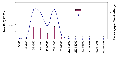
Figure 13 Areal distribution at different altitude (The area in
a logarithmic scale)
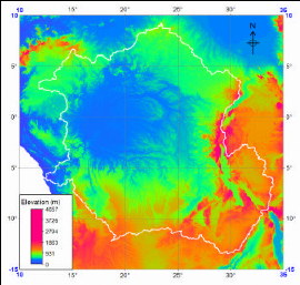
Figure 14 DEM visualization map for Cental Africa. The defined
colored polygone delineated the Congo River basin.
Table 4 Summarised Statistics for the DEM
|
Elevation
|
npix
|
npixpct
|
npixcum
|
npcumpct
|
Area (Km square)
|
|
0-100
|
46440
|
0.65
|
41461805
|
553
|
46956
|
|
101-200
|
88017
|
1.24
|
47682206
|
636
|
88994
|
|
201-500
|
1984879
|
27.92
|
342086982
|
4563
|
2006916
|
|
501-750
|
1770620
|
24.91
|
869454897
|
11598
|
1788574
|
|
751-1000
|
901295
|
12.68
|
1183992072
|
15794
|
911302
|
|
1000-1500
|
2006891
|
28.23
|
3176337475
|
42371
|
2029172
|
|
1501-2000
|
274325
|
3.86
|
3693851852
|
49274
|
277371
|
|
2001-2500
|
28808
|
0.41
|
3738833270
|
49874
|
29128
|
|
2501-3000
|
6081
|
0.09
|
3716166768
|
49572
|
6149
|
|
3001-3500
|
1168
|
0.02
|
2840777253
|
37895
|
1181
|
|
3501-3999
|
467
|
0.01
|
1866541342
|
24899
|
472
|
|
4000-4005
|
n/a
|
0.00
|
-
|
-
|
|
|
4006-4657
|
114
|
0.00
|
607211659
|
8100
|
115
|
PS: npix= number of pixels, npixpct= percentage of number of
pixels, Npicum = cumulated percentage of number of pixels. In colone 2, the
pixel numbers with -9999 elevation value are ignored.
4.3.2 Flow direction map
This step comes after fill-sink step. The filled DEM was then
used to find the flow direction map using standard D-8 algorithm (Figure 15).
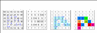
Flow direction is calculated for every central pixel of input blocks of 3 by 3
pixels, each time comparing the value of the central pixel with the value of
its 8 neighbors. The steepest slope method was used for this study to find the
steepest downhill slope of a central pixel to one of its 8 neighbour pixels and
assign to flow directions.
Calculating flow directions from a DEM (steepest slope)
Output flow direction map
Calculating flow accumulation
Output flow accumulation map
Figure 15 D-8 algorithm: Based on the output Flow
direction map, the Flow accumulation operation counts the total number of
pixels that will drain into outlets (after ILWIS 3.4 Manual)
The output map shown in Figure 16 contains flow directions
grids as N (to the North), NW (to the North West), NE (to the North East), SE
(to the South East), S (to the South) and SW (to the South West).
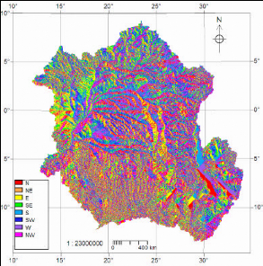
Figure 16 Flow direction map
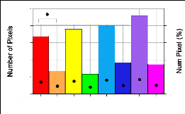
The histograms (Figure 17) indicate that the flow direction
algorithm tends to favor the cardinal directions (north, south, east and west)
over the diagonal directions (northeast, northwest, southeast and southwest).
For the entire dataset (rectangular area) 63 % of grids cells had flown in a
cardinal direction as compared to 37 % diagonals. This indicates that the flow
direction algorithm used in the model is predisposed in favor of flow through
the cardinal directions. The same observation was done in previous study on the
basin (Kwabena, 2000).
600000
400000
200000
700000
500000
300000
N NE E SE S SW W NW
Flow Direction Orientation
CB_Fdir_filled x Number Pixel Perc CB_Fdirjilled x NPix
60
40
20
80
0
100
Figure 17 Histogram of Flow Direction for Central
Africa
Table 5 Summarised statistics for the Flow direction grid
map in the area of study.
|
Flow direction Orientation
|
Number Pixel
|
% Number pixels
|
Area (Km2)
|
|
E
|
579477
|
15
|
579477
|
|
N
|
536518
|
14
|
536518
|
|
NE
|
334119
|
9
|
334119
|
|
NW
|
372838
|
10
|
372838
|
|
S
|
600426
|
16
|
600426
|
|
SE
|
314363
|
8
|
314363
|
|
SW
|
382729
|
10
|
382729
|
|
W
|
658407
|
17
|
658407
|
|
Min
|
314363
|
8.3
|
314363
|
|
Sum
|
3778877
|
100.0
|
3778877
|
4.3.3 Flow accumulation
The flow direction grid developed at the previous step is then
used as input data for Flow Accumulation grid calculations. The flow
accumulation map contains cumulative hydrologic flow values that represent the
number of input pixels which contribute any water to any outlets; the outlets
of the largest streams (drain, river) will have the largest values which is
3778906 for the Congo River basin. The grid generated (Figure 18) has a minimum
of 1 and a maximum of 3778906 pixels values for computed flow accumulation
matrix.
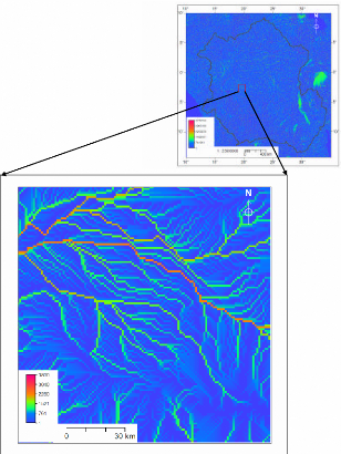
Figure 18 Flow Accumulation map; on top: Entire basin, on
bottom: A selected area
4.3.4 Drainage network extraction and
ordering
The Drainage Network Extraction operation extracts a basic
drainage network (raster map). As input it is required the output raster map of
the Flow Accumulation operation and a defined threshold value. A threshold
value, i.e. a value for the minimum number of pixels that are supposed to drain
into a pixel to let this pixel remain as a drainage in the output map; the
larger is this value, the fewer drainages will remain in the output map.
Depending on the flow accumulation value for a pixel and the threshold value
for this pixel, it is decided whether true or false should be assigned to the
output pixel. If the flow accumulation value of a pixel exceeds the threshold
value, the output pixel value will be true; else, false is assigned. A
threshold value of 1000 (number of pixels) is used in this process and 1752
stream segments are identified in the Congo River Basin masked (Figure 19).
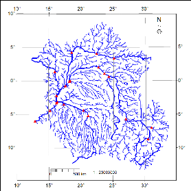
Figure 19 Stream network map masked by the boundary of the Congo
River Basin 4.3.5 Catchment and Sub-Catchments extraction
During the Catchment extraction operation, 3435 sub-catchments
were extracted. Using the Cross operation 1752 sub-catchements only (Figure 20)
were selected; each of them corresponding to a single stream segment from the
Drainage network ordering operation. This operation delivers an output raster
map, an output polygon map and an output attribute table.
The attribute table (appendix 6) andd Table 6 summarises
information for each catchment, such as the area, longest flow path, density,
and perimeter of catchment, the total upstream area. Figures 21-22 show 5
sub-catchments corresponding to 5 defined outlets namely Sangha, Ubangi, Kasai
and Lualaba. The Congo sub-catchment is generated with the residual area.
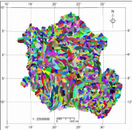
Figure 20 Extracted sub-catchment map in the Congo
Basin
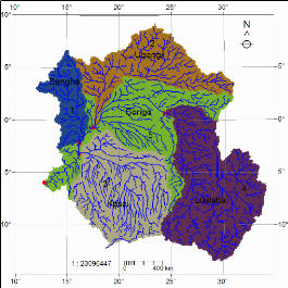
Figure 21 Merged sub-watershed with stream network and
majors outlet of the CRB
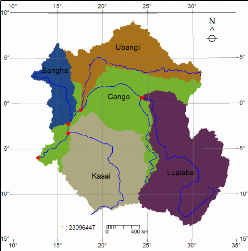
Figure 22 Longest flow path map overlayed on the
sub-watersheds of the CRB
4.3.6 Overland Flow map
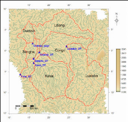
Figure 23 Overland flow distribution in the study
area
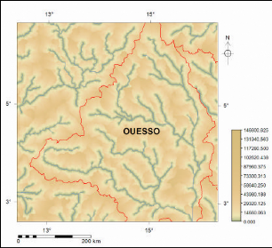
Figure 24 Overland flow distribution in the Ouesso
sub-watershed
| 

